Training Lab · Export

Take the skill home.
One file, no training stack.

Everything the robot learned in simulation ends up in a single ONNX file: the policy network, the observation normalisation and the action limits. On the robot you need onnxruntime and numpy, a loop that reads sensors at the right rate, and a healthy respect for the gap between simulation and reality.

Teach a new trick Read the docs

ONNX opset

random inputs in the verification

10⁻³

max allowed difference vs the original

libraries on the robot

1The artifact

A deterministic policy with its normalisation inside

Export traces the trained actor network into ONNX, the open format for neural networks. The critic, the optimiser state and the exploration noise are left behind; what remains is a pure function from observation to action.

obs

float32 [batch, obs_dim] · raw values, training order

normalise

(obs − mean) / √(var + 1e-8), clip ±10

actor MLP

64 → 64, tanh · the trained policy

mean action

no sampling: deterministic

clip

to the action-space bounds

action

float32 [batch, act_dim]

Inside the exported graph (orange: part of the graph). Input obs and output action have a dynamic batch dimension.

Deterministic

For PPO the output is the mean of the policy’s action distribution: the same action model.predict(obs, deterministic=True) returns. Same observation in, same command out.

Normalisation baked in

The frozen running mean and variance from training become the first layer, with the same ±10 clip. You feed raw sensor values, never pre-scaled ones.

Clipped actions

The output is clipped to the action-space bounds inside the graph, so it is always a valid command vector for the task’s action space.

Any completed run can be exported; the Export page features the best one (highest mean return). Downloads are named <task>_run<id>_PPO.onnx, and a policy of this size is well under a megabyte.

2Trust, but verify

Checked against the original, described by its metadata

An export that silently differs from the trained policy would be worse than none. So every export of a completed run is checked before you can download it.

Verification

The model must pass the official onnx.checker.
16 random observations are run through both the ONNX file (with onnxruntime) and the original Stable-Baselines3 policy (with the same normalisation).
If any action differs by more than 0.001, the export is rejected. The largest difference is recorded as max_abs_diff_vs_sb3; in practice it is floating-point rounding.
The file’s size and SHA-256 checksum are computed, so you can confirm the file on the robot is the one you exported.

Field	Meaning
`input · output`	Tensor names, dtypes and shapes: obs [1, obs_dim] and action [1, act_dim].
`action_space`	Low and high bound of each action value.
`obs_normalization · obs_clip`	vecnormalize and 10.0 when statistics are baked in.
`robot_model · env_* · run_id`	Which robot, task, task version and run the policy came from.
`verified · max_abs_diff_vs_sb3`	Result of the comparison with the original policy.
`size_bytes · sha256`	Integrity of the file.
`browser_sim`	Whether the browser can run it live, with the observation recipe or the reason it can’t.

policy metadata · example values

{
  "format": "onnx",
  "opset": 17,
  "algorithm": "PPO",
  "deterministic": true,
  "input":  { "name": "obs", "dtype": "float32", "shape": [1, 26],
              "note": "RAW environment observation; normalisation is baked into the graph" },
  "output": { "name": "action", "dtype": "float32", "shape": [1, 6],
              "note": "clipped to action space bounds" },
  "action_space": { "type": "Box", "low": [-1.0, …], "high": [1.0, …] },
  "obs_normalization": "vecnormalize",
  "obs_clip": 10.0,
  "robot_model": "Walker2d", "env_id": 12, "env_slug": "kick-the-ball",
  "env_version": 3, "run_id": 42, "exported_by": "kualia.ai",
  "verified": true, "max_abs_diff_vs_sb3": 2.4e-07,
  "size_bytes": 41213, "sha256": "…",
  "browser_sim": { "supported": true, "recipe": { … }, "verify": { "steps_checked": 40 } }
}

The metadata is embedded in the ONNX file itself (metadata_props, one JSON value per key), saved as JSON next to it on the server, and shown on the Export page. On the robot, read it back with sess.get_modelmeta().custom_metadata_map.

3Deployment

Running it on the robot

The integration is a fixed-rate loop: build the observation vector, run the policy, send the commands, wait for the next tick. The hard part is the first line, making the observation match simulation exactly.

robot_loop.py

# On the robot: pip install onnxruntime numpy   (onnxruntime 1.16+ for opset 17)
import json, time
import numpy as np
import onnxruntime as ort

sess = ort.InferenceSession("kick-the-ball_run42_PPO.onnx", providers=["CPUExecutionProvider"])
meta = {k: json.loads(v) for k, v in sess.get_modelmeta().custom_metadata_map.items()}
OBS_DIM = meta["input"]["shape"][1]

HZ = 125                      # the task's control rate, shown on the Export page
DT = 1.0 / HZ


def policy(obs):
    x = np.asarray(obs, dtype=np.float32).reshape(1, OBS_DIM)   # RAW values, training order
    return sess.run(["action"], {"obs": x})[0][0]              # normalised + clipped inside


next_tick = time.perf_counter()
while not emergency_stop():            # your code
    a = policy(read_observation())     # your code: same layout and units as in simulation
    send_commands(to_ctrl(a))          # your code + the mapping below
    next_tick += DT
    time.sleep(max(0.0, next_tick - time.perf_counter()))

Keep the loop at the task’s control rate. The Export page shows it; for the built-in robots it ranges from 20 Hz (Ant, HalfCheetah) to 125 Hz (Hopper, Walker2d).

Match the observation

Same order as in training: joint positions, then joint velocities, then world objects relative to the robot’s base.
Same units: metres, radians, rad/s.
Same conventions: the base’s world x/y is not in the observation; joint velocities were clipped to ±50 and object velocities to ±20.
Objects mean you need to sense them on the real robot too, for example a ball position from a camera.

4Actuation

From policy output to actuator command

On kualia’s runtime every actuator is normalised to [−1, 1] during training and mapped linearly onto its control range. Do the same on the robot and the command means what it meant in simulation.

Example: a position servo with a control range of −0.8 to 0.8 rad.

actions → actuators

# kualia runtime: each action value in [-1, 1] spans one actuator's control range,
# exactly as in simulation (a joint target for a position servo, a torque for a motor).
CTRL_LOW  = np.array([...])   # per actuator: MJCF ctrlrange (centred on the standing keyframe if the model has one)
CTRL_HIGH = np.array([...])

def to_ctrl(a):
    a = np.clip(a, -1.0, 1.0)
    return CTRL_LOW + 0.5 * (a + 1.0) * (CTRL_HIGH - CTRL_LOW)

On the realistic Menagerie robots (and uploaded models that ship a keyframe) each position actuator’s range is shifted to centre on the standing keyframe, width unchanged, so an action of 0 holds the standing pose. Use those shifted ranges for CTRL_LOW / CTRL_HIGH; when the task supports browser simulation, the metadata’s browser_sim recipe lists them exactly.

Gymnasium-route tasks on the classic robots use the robot’s own action space instead; the bounds are in the metadata’s action_space. For a position servo the value is a joint target, for a motor a torque, so check which one your real actuator expects.

5Reality check

Mind the sim-to-real gap

A policy is only as good as the simulation it trained in. Real motors have latency and backlash, friction differs, batteries sag and sensors are noisy. Expect differences, and design the first tests so they are harmless.

Start at low power

Low gains, low speed limits, reduced torque. Raise them only once the behaviour looks right.

Emergency stop in reach

A physical e-stop or a kill switch that cuts motor power, and people out of the robot’s reach.

Suspend or tether first

Run a legged robot lifted or on a harness before it bears its own weight.

Watch the timing

If a tick is late or a sensor read fails, hold a safe pose instead of acting on stale data.

a guard for first tests

# First hardware tests: a guard between the policy and the motors.
MAX_DELTA = 0.05            # largest change per control step, in actuator units

prev = None
def guard(ctrl):
    global prev
    ctrl = np.clip(ctrl, SAFE_MIN, SAFE_MAX)            # your own, tighter limits
    if prev is not None:
        ctrl = prev + np.clip(ctrl - prev, -MAX_DELTA, MAX_DELTA)
    prev = ctrl
    return ctrl

Clamp to your own joint limits and rate-limit changes while you test. A guard changes the dynamics the policy learned, so remove or loosen it once the robot behaves.

What varies in training today

Small random noise on joint positions and velocities at every reset.
Random placement (jitter) of movable world objects.
Task-level variation alia writes, such as a randomised target or command picked in on_reset().

The robot’s physical parameters (masses, friction, motor strength) stay fixed: kualia does not randomise dynamics today. Plan real-world tests with that in mind.

Control rate matters

If your robot’s loop runs at a different rate than the task, retrain with CONTROL_HZ set to the real rate rather than resampling actions.

6Before the hardware

The same file runs in your browser

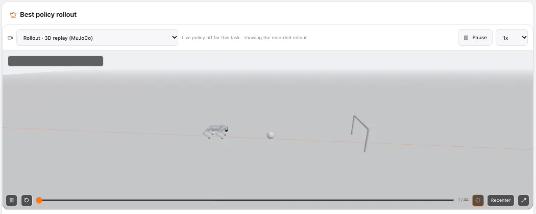
The Export page loads the exact ONNX file you download into the browser simulator: MuJoCo in WebAssembly plus onnxruntime-web, driving the robot in real time. Push it, watch it recover, and only then move to hardware.

Try the exported policy on the Export page: the policy acts in the same composed world it trained in, objects included.
During training, the newest checkpoint from 25 % on is exported to ONNX on request and runs live on the Training screen, refreshing as new checkpoints are recorded.
The Export page’s Browser simulation line says whether the task can run live, with the reason when it can’t (custom observation features, action remapping, a different control period).
ONNX is a standard format, so the policy runs in your own web or desktop tools too.

onnxruntime-web

import * as ort from "onnxruntime-web";

const session = await ort.InferenceSession.create("/kick-the-ball_run42_PPO.onnx");
const obs = new Float32Array(26);              // raw observation, training order
const out = await session.run({ obs: new ort.Tensor("float32", obs, [1, obs.length]) });
const action = out.action.data;                // Float32Array, one value per actuator

Live policy — The exported policy running live in the browser. Push the robot to test robustness.

7The handoff

What you can take with you

The Export page packages everything a robot-side integration needs, and the Plan page shows the task the policy learned.

The ONNX policy

Download File on the Export page. Deterministic, normalisation inside, verified.

Metadata & checksum

Input and output schema, control rate, normalisation, and the SHA-256 hash to copy.

Runtime snippet

Copy Runtime Instructions gives a minimal onnxruntime loop for your file’s shapes and rate.

The task code

The generated Gymnasium task is plain Python; read and copy it on the Plan page.

The file is the handoff

Direct push to a robot runtime is on the roadmap. Today you copy the ONNX file to the robot (scp, USB, your robot’s tooling) and run it with onnxruntime.

Questions

Do I need PyTorch or Stable-Baselines3 on the robot?

No. The file is a plain ONNX graph. onnxruntime and numpy are enough, on a laptop, a Raspberry Pi or a Jetson, as long as the runtime supports opset 17 (onnxruntime 1.16 or newer).

Do I have to normalise the observation myself?

No, and you must not. The training mean and standard deviation are inside the graph. Feed raw values in the same order and units as in simulation.

Why is the exported policy deterministic?

During training PPO samples actions around a mean to explore. On a robot you want the same observation to give the same command, so the export keeps only the mean action, exactly what Stable-Baselines3 returns with deterministic=True.

My robot’s control loop runs at a different rate. Can I resample?

Don’t. The policy learned dynamics at one control period. Ask alia to retrain with CONTROL_HZ set to your robot’s real rate instead.

Can I export a run that is still training?

The Studio exports completed runs. While a run trains, the newest checkpoint from 25 % on is exported on request so the browser can run it live; that interim export skips the verification step.

Can kualia push the policy to my robot directly?

Not yet. Direct push to a robot runtime is on the roadmap; today the handoff is the ONNX file.

Train it here. Run it there.

A first 10K-step try costs $1, and a failed run costs nothing.

Open Studio How it works

Next · Training LabReinforcement learningThe learning loop, PPO, rewards and how runs are judged.Also in the labSimulationMuJoCo physics, robots, worlds and the browser simulator.

Take the skill home.One file, no training stack.